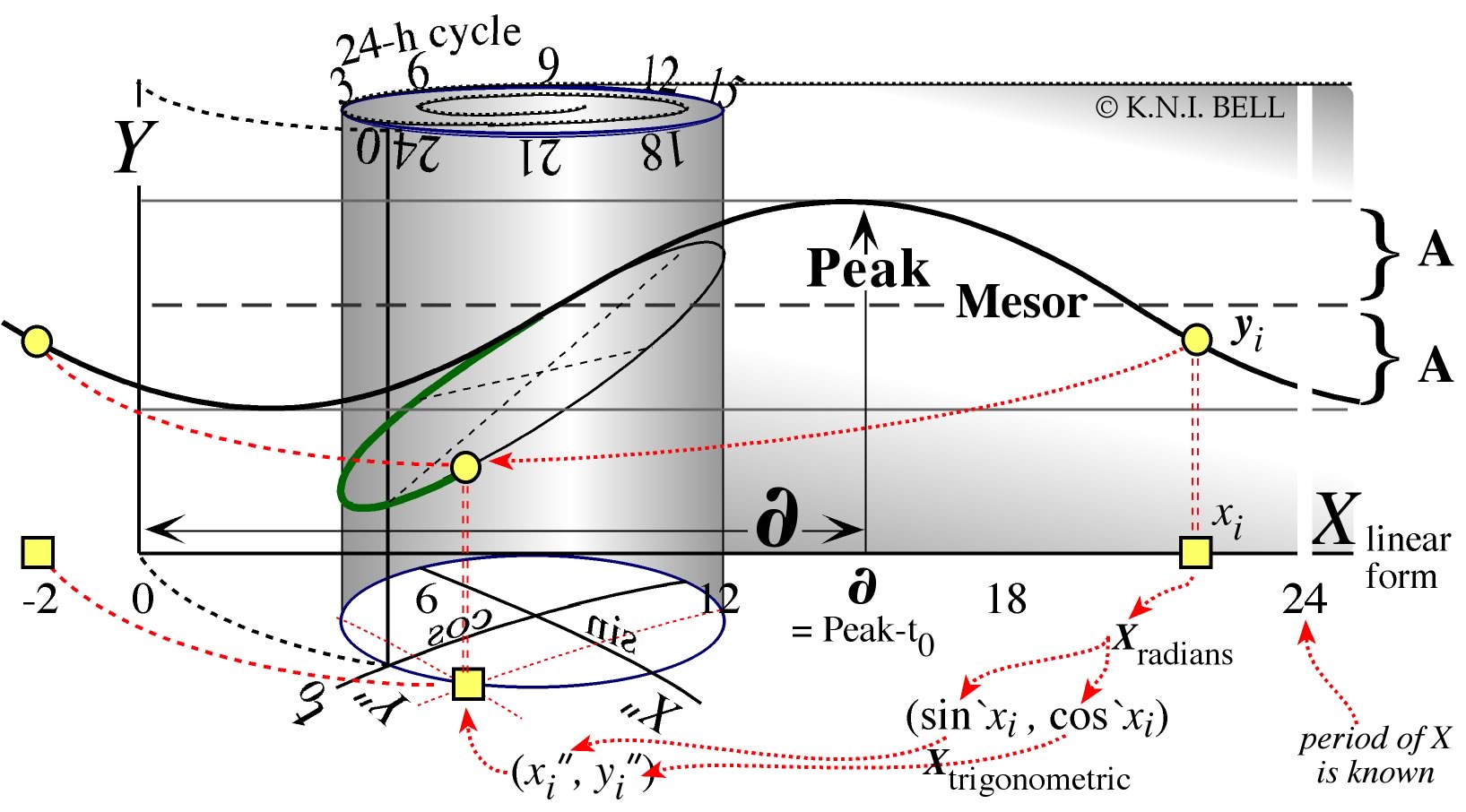
Figure 6-3. Conceptualising
periodic regression: Y vs. circular X. A flat graph
of periodic data in a wave-like pattern is “printed” onto
a cylindric graph rolled across it, or vice versa. The x-axis
of the flat graph is cyclic format of circular X (this example
has period of 24 units), while the cylinder base has the (sin`x,cos`x)
coordinates (trigonometric format) of X, the transforms that
are essential for analysis. The cylinder has radius 1.0 (unit circle).
Mesor, Phase
angle (∂)
of the peak, and Amplitude (A) are marked.
In more detail: a sinusoidal function, or data, is visualised
as a sinusoidal
curve ‘peeled’ or ‘printed’ from
a flat plot onto a cylinder (or vice versa). A sine curve results
from the intersection of a flat plane and a cylinder; that's why it
is the simplest possible repeating curve and the reasonable (most parsimonious)
periodic model form to assume (examination of residuals will show whether
other models need to be explored). Periodic regression is easiest to
conceptualise by visualising how the data actually exist on the cycle.
For now, imagine the data are temperatures
(Y) over (X) the 24h daily cycle. X (0≤x≤24)
is a circular variable; we can tell it's circular because on the cycle
24=0. Midnight is 24h or 0h*. Same thing. In fact, in the cycle,
any angle plus one complete revolution is the same angle, e.g. time xh
= xh+24, 10 a.m. plus one day is still 10 a.m. If the
number of days, or number of turns of a screw, or the number of years,
etc., is important then that number is usually treated as a linear
variable separate from, or even instead of, the angle.
* For simplicity there we only
used whole hours; why? Because the so-called 'military' or '24-h'
time
as commonly used is not
a proper
number. It's two different kinds of number stuck together: 1025h
does not mean 10.25 hours, it
means 10hours25minutes, or 10+25/60 hours, =10.41666 hours. But the regularity
still prevails:
on
the
daily
cycle, 10.4166h=34.4166h ... if plotted, the angle is the same, and the sines
and cosines are the same. That added 24h is one whole day, and if the data contain
time indices spanning several days and various times of day, and if the day number
is
important to include in analysis it must be treated as
a linear variable while the times of day are (unavoidably) circular.
For
more
on
time
measurement conventions, see the ISO 8601 standard. Our normal time language
such as "twenty
to
five" or "four-thirty" is actually a host of conventions, only in special cases
(whole hours)
being proper numbers.
Circular variables require special
handling so that, in effect, the analysis
does not
treat x=24
differently from x=0. We can't simply regress Y vs. X (0≤x≤24);
that would give us nonsense, partly because on that cycle 24=0, and
because that would fit a straight line rather than a repeating function.
Instead, we have to first decompose the circular X into its
linear components: then we can analyse Y
vs. the
proper sine and cosine of X. We indicate the proper sine etc
by a following grave [pronounced grahv] accent, as when we write Y
= B0 + B1*sin` X + B2*cos`X. The grave accent ` indicates
"proper" sine and cosine as obtained after converting X to
degrees or radians (units that allow taking sine or cosine). Using
the grave accent ` lets us focus on the issue of interest rather than
the machinery and units. This notation is quicker and more general
than writing Y
= B0 + B1*sin(X*2*π/k)
+ B2*cos(X*2*π/k), or --- because this long
form uses radians and doesn't acknowledge that we would equally well
use other units --- writing X*360/k instead
of X*2*π/k if using degrees instead of radians,
where k is
the number of units in the cycle (here 24 h).
A
further notational economy, useful when discussing coordinates of vectors
implied by circular variables, is x" and y" for sin` X and cos`X,
i.e. the pair transforms that 'translate' X, which is a circular
index variable (time, direction, etc.), into linear components that
can be analysed in a regression. There may be other Xs
that are not circular and these are not transformed but can exist in
the
same regression
with circular Xs.
Do not confuse
y" with the independent variable Y. We first
map the cycle (X)
as a circle at the base of the figure. To save us trouble, we define
the
the circle
as having radius=1.
Now, the circle representing X has two dimensions (sine and cosine, which
we can call X" and Y"), and the positions of each observation
are readily seen to equate to coordinates that equate to the proper sine and
cosine of X. Next, we map Y as height above the circle (alternative
representations are possible, e.g. the polar plot), but using height lets us "print" the
data from its cylindrical arrangement onto a flat page, or vice versa, as the
diagram shows. In a publication the data might often be plotted in the flat configuration,
i.e. Y vs. a linear format of X, or as a polar plot, but
rarely in this kind of perspective cylindrical form that links them all.
The proxy variables x" and y" thus
are
transforms of the independent variable X (pseudolinear, e.g. degrees of
a circle, hours of a day, days of a year) axis. These proxy variables form axes
of coordinate
space (indicated by the double-prime mark ") on which the angles of the
linear X variable are expressed; this ‘trigonometric’ is
required for analysis of a cycle (e.g. by regression).
Mesor, Phase, and Amplitude (A) are the three key parameters
of a cycle. These relate to the graph, with the mesor being at the center
of
the
intersection of plane and cylinder or halfway between the lowest and highest
expected values,
the
phase
being
the
angle or direction corresponding to the highest expected value, and amplitude
being
the
difference
between the
mesor and the highest or lowest expected value.
Although we usually obtain sine and cosine from tables or
functions on our calculators, it's nice to know that we could do it graphically.
If
we
declare the
radius
of
the
rolled-up
graph
to be 1.0 and thus create a unit circle on which any angle can be expressed,
and
if we then draw
coordinate axes X" and Y" through the centre of the unit
circle,
a
point
(x",y")
represents the sine (X"=sin`x=sin(X*2π/k,
where k is the number of angular units into which we've divided the
cycle of interest, e.g. 360 degrees, or 24h, or 365 days) and cosine
(Y"=cos`x=cos(X*2π/k))
transform of the original time scale. Expressions like sin`x thus
use the grave mark to mean "proper", i.e. the proper sine, taken
after x has
been properly transformed to a standard angular system like radians. Thus
(x",y")
are paired transforms of the periodic X variable, in this example
a 24h cycle, and the transforms are proxy X-variables on which a
regression can be conducted.
The
phasing
of the data peak relative to the nominal zero of the cycle is ∂ = P-t(0). ∂ can
be identified iteratively, or graphically as below, or explicitly by regression
using X" and Y" to model the variation in the dependent
variable Y. Statistical significance is a separate issue from fitting
the function, and cautions against some tempting errors are given in the
book.